The Ecstasy of Gold: Multivariate Interpolation with Kriging

Reading Time: 21 min 35 sec

In the early dawn of the 1960s, nestled deep in the heart of South Africa, a mining engineer by the name of Daniel Gerhardus Krige was confronted with a peculiar conundrum. His task was to meticulously choose segments—or “panels”— within two gold mines that would yield more value than the cost of the extraction itself. ¹

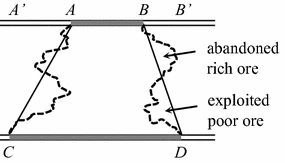
A panel, you see, was an area partitioned using some arbitrary method on the geographical map of the mine. For instance, it could be the trapezoid marked ABDC as shown in the illustration. The real challenge for Krige lay in unlocking the value of these panels: determining the average gold grade in each one.

While one could argue that this was an estimation game, the only real evidence at Krige’s disposal were the sampled gold grades from the narrow veins labelled AB and CD, plus an average gold grade for the entire mine.

The popular method of the era relied on averaging these sample grades. However, Krige had noticed a worrisome pattern - this method often gave an overstated estimation of the gold grade. This method was imperfect, for it overlooked the poor quality ores concealed within the panel, and disregarded the rich ores that lay beyond its boundaries. Quite simply, the mining map did not match the natural distribution of gold vein richness.

To balance this bias, Krige had a brainwave. He thought: why not offset the average grade of the sample data with the average grade of the whole mine? He could assign a weight \(\lambda\) to the sampled average, and \(1-\lambda\) to the total average, with the weight being determined using a linear regression on all the panels.

Meanwhile, across the ocean in France, mining researcher Georges Matheron was inspired by Krige’s work. Matheron saw value in not just removing bias, but also minimizing the estimation variance. He introduced the idea of assigning a weight to each sample, where for any selected point of interest within the panel, the value was interpolated from the samples using a weighted average. Matheron, in a nod to Krige, christened this method “Kriging”.

Kriging, over the course of six decades, became a cornerstone principle in geographical and multivariate interpolation problems. It emerged, quite literally, as a tool for unearthing gold, becoming as vital to the trade as a miner’s lamp or a sturdy wagon.

Imagine having a lamp which provides temporary light and can only illuminate a restricted area of a mine. Now, visualize gaining the skill to krig - a tool that will empower you to mine anything, anytime, anywhere without even seeing the ores. How cool is that?

It’s the purpose of this investigation to show you the mechanisms behind kriging, and how it’s applied for any multivariate interpolation task.

Problem

Given \(N\) \(n\)-dimensional data points \(\mathbf{x}_1, \cdots \mathbf{x}_N\), and their observed values from a function \(y_i=f(\mathbf{x}_i)\), we would like to obtain an interpolation function \(g(\mathbf{x}_i)\) s.t. it can approximate \(f\) while passing through all \(\mathbf{x}_i\) exactly. Moreover, we want it to be relatively smooth to the extent that it has continuous values and first derivatives.

A straightforward thought is: can we define each point on \(g\) as a linear combination of the known values? With this assumption, for each point we can define a set of weights \(w_1, \cdots, w_N\) to express this combination, which satisfies the interpolation requirements above.

Our interpolation \(g\) can then be expressed as:

\[\hat{y}=g(\mathbf{x})=\frac{\sum^{N}_{i=1} w_i y_i}{\sum^{N}_{i=1} w_i}\]

The denominator is to normalize the weights s.t. they sum to 1, forming an unbiased estimation. Although it turns out this step is seldom needed for the soundness of most methods.

It turns out that there are many methods to determine this linear combination, such as the unweighted average mentioned in the introduction, IDW(Shepard Interpolation) and RBF. Essentially, we are just putting additional assumptions on the combination to help obtaining proper weights. For example, we could assume that it minimizes some sort of energy function (e.g. thin-plate splines RBF), or the weights are directly defined by some pairwise distance function (e.g. IDW).

One particularly interesting question is: instead of determining a proper assumption from observations of applied experiments, which are what the above methods are doing, can we assume there exists a theoretically “best” interpolation scheme within the scope of using linear combination, and use this scheme?

Well, the question itself implies that we need some common metrics to judge the goodness of fit of \(g\) on \(f\). What does that remind you of? The mean and variance!

So what could be a good criteria to say that a linear combination based interpolation is the “best” in its results by looking at the mean and variance relationship between it and the target function? We could require it to be a best linear unbiased predictor (BLUP) s.t.:

1. \(Var(y - \hat{y})\) is minimized,
2. \(\mathbb{E}[y - \hat{y}]=0\),

for each observation-interpolation pair, provided that \(y\) is already rid of observation error.

Our problem is then to find such a linear combination that is a BLUP, while also satisfying the interpolation requirements.

Constraints

To satisfy the requirement of unbiased estimation, we need to ensure that our weights sum to identity:

\[\sum^n_{i=1}w_i=1.\]

Notice that with this inherent enforcement, it’s unnecessary to do the normalization again in the problem definition.

Assumptions

Assumptions of A Random Field ²

Before we start solving the Kriging problem, we need to make some assumptions(restrictions) on the randomness of the field in interest, i.e. the field \(R\) that all data points reside in. Without these assumptions, the computation of Kriging becomes intractable.

Given the observed \(N\) data points in an \(n\)-dimensional space, we can assume that each of them completes one of many possible realizations of a random process. This also implies that uncollapsed uncertainty lies in the unobserved points elsewhere.

This assumption defines a random process for each point. These random processes are intractable as they are infinite. To further reduce the problem, we can assume that:

1. Each random process has the same form.
2. There exists a spatial dependence among points, making them dependent on each other.

With these additional assumptions, we can construct a random process over the whole random field \(R\).

We still need to express the set of random variables in \(R\), which contains the point positions and the point evaluations. For the evaluations, we coin a regionalized variable \(Z={Z(\mathbf{x}), \forall \mathbf{x} \in R}\). Together with the point positions, they characterize the random field.

Let’s pause for a bit and think about what we have so far: an assumed random field, and a single realization for each observed data point of this random field.

Our objective is to have a BLUP. From the perspective of our random field, this means that:

1. We must estimate the expected values of the random process at each point to be the same with the ground-truth process.
2. We must estimate the autocorrelation of the regionalized variable to be the same with the ground-truth process.

By autocorrelation, we just mean a description of how the observations of \(Z\) are correlated with each other.

If you feel a bit clueless for obtaining these two steps, don’t worry! This just indicates that we are not making enough assumptions of our random process to reduce the problem even further. In other words, the process is still too “indeterministic” for us to approach.

We are gonna introduce two simplifications as the first and second order stationarities for the rescue.

First-order Stationarity

At each sampled point, we have only one realization of the random process, while infinitely many such realizations are possible.

To make a reasonable estimation, we could assume that the expected values at all points are the same in the random field. This is the first-order stationarity.

In certain situations, we might want to relax this assumption a bit to consider for a more complex estimation. The objective is always to deny first-order stationarity and allow an arbitrary dynamic modeling in the process. Consider these two cases:

1. We observe the expected values to be different in different regions of the field.
2. We observe a trend across the field’s regions.

An intuitive idea is that we can apply a decomposition of stationarity and dynamics: we explicitly estimate the trend or regional patterns in the expected values first, as a basis estimation, and then estimate the stationary residuals that lead to a full estimation.

The basis estimation needs an auxiliary estimator, which does a trend/region-conditioned prediction. The stationary residuals are just estimated by simple kriging.

Depending on the applied conditions of the auxiliary estimator and the amounts of such estimators, we have universal kriging (UK), kriging with external drift (KED) and regression kriging (RK). These methods are highly similar variants, and a comparison can be found on the wikipedia.

We are only gonna consider the simple first-order stationary case here, which leads to ordinary kriging (OK).

Second-order Stationarity

As an analogy, autocorrelation is just correlating one probable reality with another in different “parallel universes”, where each universe has a specific random field realization.

As each sample point can be regarded as a different realization of the field random process, the autocorrelation of the random variable \(\mathbf{z}\) can be expressed as the covariances between different sample points.

Our target is now to estimate this covariance between any two points in the field:

\[\hat{C} \left( \mathbf{x}_{1} ,\mathbf{x}_{2} \right) =\mathbb{E} \left[ \left( Z\left( \mathbf{x}_{1} \right) -\mathbf{\mu } \left( \mathbf{x}_{1} \right) \right) \cdot \left( Z\left( \mathbf{x}_{2} \right) -\mathbf{\mu } \left( \mathbf{x}_{2} \right) \right) \right] .\]

Notice that there is also an underlying assumption here that the covariance is only conditioned by the spatial relationship.

With the assumption of first-order stationarity, we could simplify the expected value computation for each point:

\[\hat{C} \left( \mathbf{x}_{1} ,\mathbf{x}_{2} \right) =\mathbb{E} \left[ \left( Z\left( \mathbf{x}_{1} \right) -\mathbf{\mu } \right) \cdot \left( Z\left( \mathbf{x}_{2} \right) -\mathbf{\mu } \right) \right] .\]

One more problem remain: in the autocorrelation we also need to estimate variance. This is defined by a point’s covariance on itself:

\[\sigma^{2} =\hat{C} \left( \mathbf{x}_{i} ,\mathbf{x}_{i} \right) =\mathbb{E} \left[ \left( Z\left( \mathbf{x}_{i} \right) -\mathbf{\mu } \right)^{2} \right] .\]

But we only have one realization for the expectation. How do we estimate the variance?

We can assume that the variance is the same at all points in the random field. This is part 1 of the second-order stationarity.

With this assumption, the variance for any point could be estimated from the variance considering all observed data points.

This is nice, but how much work needs to be done to get the covariance between all points? Apparently, for any arbitrary point we need to correlate it with all the points in the field, which yields a huge complexity. If we only resolve to the observed data points, then only one realization is given for each point pair, which is not sufficient for the estimation.

Therefore, part 2 of the second-order stationarity is to assume the covariance only depends on the separation between two points.

To recapitulate, we now have the following two assumptions:

1. The variance is the same at all points in our random field.
2. The covariance only depends on the separation between the given two points.

If we define this separation to be \(\mathbf{h}\), then we can write the covariance estimation as:

\[\begin{gathered}C\left( Z\left( \mathbf{x} \right) ,Z\left( \mathbf{x} +\mathbf{h} \right) \right) =\mathbb{E} \left[ \left( Z\left( \mathbf{x} \right) -\mathbf{\mu } \right) \cdot \left( Z\left( \mathbf{x} +\mathbf{h} \right) -\mathbf{\mu } \right) \right] \\ =\mathbb{E} \left[ Z\left( \mathbf{x} \right) \cdot Z\left( \mathbf{x} +\mathbf{h} \right) -\mathbf{\mu }^{2} \right] \\ \equiv C\left( \mathbf{h} \right) .\end{gathered}\]

This is termed autocovariance of the regionalized variable, (auto just means self here, nothing special). For convenience of our later discussion, let’s define two more entities:

The autocorrelation is just the normalized version of the autocovariance:

\[\rho \left( \mathbf{h} \right) =\frac{C\left( \mathbf{h} \right) }{C(0)} .\]

The semivariance is the residual of the covariance with the variance.

\[\gamma \left( \mathbf{h} \right) =C\left( 0\right) -C\left( \mathbf{h} \right) .\]

Intrinsic Hypothesis

We are now comfortable with the covariance estimation. Nevertheless, a restriction has been posed by our assumptions of second-order stationarity. Now we must require the following conditions to hold:

1. The covariance must exist.
2. The variance must be finite, i.e. \(C(0)\) is defined.

Particularly in application, we can observe that the covariance increases without bound as the random field’s area increases. This has an intuitive, albeit unexamined, explanation: a local random variable can become less stable as the range of observation widens, and since covariance is not normalized as correlation, this ultimately leads to a boundless accumulation.

We can mitigate this effect a bit by considering the differences between covariances instead of the values themselves, thus avoiding large values. This is why we have defined the semivariance above.

Moreover, we can add one more assumption: covariances are bounded in a small region.

These two assumptions constitute the intrinsic hypothesis. By this hypothesis, we are considering value differences instead of values everywhere. The assumption of finite covariances are thus relaxed. We only need to make sure the differences are finite.

For example, the covariances of values can be expressed as the following variances of differences:

\[Var\left[ Z\left( \mathbf{x} \right) -Z\left( \mathbf{x} +\mathbf{h} \right) \right] =\mathbb{E} \left[ \left( Z\left( \mathbf{x} \right) -Z\left( \mathbf{x} +\mathbf{h} \right) \right)^{2} \right] =2\gamma \left( \mathbf{h} \right) .\]

Modeling Semivariance: from Empirical Variogram to Variogram Model

We now know how to estimate both the expectation and the covariances. However, there is a hidden question in covariance estimation: how do we get the evaluation of \(\gamma (\mathbf{h})\) for any arbitrary \(\mathbf{h}\), given only some observed data points, so that we can run the estimator for any arbitrary point in the random field?

To start with, \(\gamma (\mathbf{h}) \equiv \gamma (\mathbf{x}_1, \mathbf{x}_2)\). We can construct an empirical variogram from the observed data points. Essentially, this is just a table mapping some discrete values of \(\mathbf{h}\) to their evaluation \(2\gamma (\mathbf{h\pm\delta})\). The arbitrary tolerance \(\delta\) defines bins for each \(\mathbf{h}\) to fall into.

The table \(\gamma (\mathbf{h\pm\delta})\) is called a semivariogram.

A natural question at this point is: why don’t we just use the empirical semivariogram? Surely we could just apply binning for any arbitrary \(\mathbf{h}\) encountered during estimation?

Recall that by definition of a covariance, we have the following properties:

1. \(\gamma(\mathbf{h})=\gamma(-\mathbf{h})\).
2. \(\gamma(\mathbf{h}) \leq 0\).

This means that for any point of interest, its semivariogram w.r.t. the sampled points must be a symmetric and negative semi-definite matrix.

With real data, such properties almost seldom hold true. Without a proper matrix, we are bound to have numerical errors.

Therefore, the big idea is to fit a variogram model to the empirical variogram. The function of this model is chosen s.t. the properties of the semivariogram matrix always holds for estimating the value at any location in the random field.

There are many such models, to name a few ³:

1. Exponential (smoother than spherical)
2. Spherical (most commonly used)
3. Gaussian (sudden changes at some distance)
4. Matérn (for extra smoothness)

You can refer to this documentation of SciKit GStat for more details.

When direction matters, there are also directional variograms available.

Ordinary Kriging

Finally, we get to krig after all the assumptions drawn!

Derivation of the Kriging Equations

Let’s derive the mechanisms of ordinary kriging step by step. As already explained in the assumptions, ordinary krigging assumes no trends, no regional patterns and an unknown expected value of the field random process.

As a linear predictor, i.e. weighted sum of observed values, the estimation of kriging at a given point \(\mathbf{x}\) can be expressed as:

\[\hat{z} \left( \mathbf{x} \right) =\sum^{N}_{i=1} \lambda_{i} z\left( \mathbf{x}_{i} \right) .\]

Recall our objectives:

1. The estimation should be unbiased.
2. The estimation variance must be minimized.

The first objective is easy to meet. We just need the weights to sum to 1:

\[\sum^{N}_{i=1} \lambda_{i} =1.\]

The second objective can be met by minimizing the following expression:

\[\sigma^{2} \left( Z\left( \mathbf{x} \right) \right) \equiv \mathbb{E} \left[ \left( \hat{Z} \left( \mathbf{x} \right) -Z\left( \mathbf{x} \right) \right)^{2} \right] .\]

Replacing the prediction \(\hat{Z} \left( \mathbf{x} \right)\) with the defined linear combination of weights we have:

\[\sigma^{2} \left( Z\left( \mathbf{x} \right) \right) =\mathbb{E} \left[ \left( \sum^{N}_{i=1} \lambda_{i} z\left( \mathbf{x}_{i} \right) -Z\left( \mathbf{x} \right) \right)^{2} \right] .\]

Assuming the first-order stationarity, we can include the universal mean \(\mu\):

\[\begin{gathered}\sigma^{2} \left( Z\left( \mathbf{x} \right) \right) =\mathbb{E} \left[ \left( \sum^{N}_{i=1} \lambda_{i} \left( z\left( \mathbf{x}_{i} \right) -\mu \right) -\left( Z\left( \mathbf{x} \right) -\mu \right) \right)^{2} \right] \\ =\mathbb{E} \left[ \begin{gathered}\left( \sum^{N}_{i=1} \lambda_{i} z\left( \mathbf{x}_{i} \right) -\mu \right)^{2} \\ -2\sum^{N}_{i=1} \lambda_{i} \left( z\left( \mathbf{x}_{i} \right) -\mu \right) \left( Z\left( \mathbf{x} \right) -\mu \right) \\ +\left( Z\left( \mathbf{x} \right) -\mu \right)^{2} \end{gathered} \right] .\end{gathered}\]

We observe there are three terms in the expectation of last expression. For the first term, we can replace the square with a double sum:

\[\left( \sum^{N}_{i=1} \lambda_{i} z\left( \mathbf{x}_{i} \right) -\mu \right)^{2} =\sum^{N}_{i=1} \sum^{N}_{j=1} \lambda_{i} \lambda_{j} \left( z\left( \mathbf{x}_{i} \right) -\mu \right) \left( z\left( \mathbf{x}_{j} \right) -\mu \right) .\]

We can also push the expectation into each term’s summations:

\[\begin{gathered}\sigma^{2} \left( Z\left( \mathbf{x} \right) \right) =\sum^{N}_{i=1} \sum^{N}_{j=1} \lambda_{i} \lambda_{j} \mathbb{E} \left[ \left( z\left( \mathbf{x}_{i} \right) -\mu \right) \left( z\left( \mathbf{x}_{j} \right) -\mu \right) \right] \\ -2\sum^{N}_{i=1} \lambda_{i} \mathbb{E} \left[ \left( z\left( \mathbf{x}_{i} \right) -\mu \right) \left( z\left( \mathbf{x} \right) -\mu \right) \right] \\ +\mathbb{E} \left[ \left( Z\left( \mathbf{x} \right) -\mu \right)^{2} \right] .\end{gathered}\]

Some patterns emerge. We see covariances and variances everywhere in the three terms, and can replace them:

\[\begin{gathered}\sigma^{2} \left( Z\left( \mathbf{x} \right) \right) =\sum^{N}_{i=1} \sum^{N}_{j=1} \lambda_{i} \lambda_{j} Cov\left( z\left( \mathbf{x}_{i} \right) ,z\left( \mathbf{x}_{j} \right) \right) \\ -2\sum^{N}_{i=1} \lambda_{i} Cov\left( z\left( \mathbf{x}_{i} \right) ,Z\left( \mathbf{x} \right) \right) \\ +Var\left( Z\left( \mathbf{x} \right) \right). \end{gathered}\]

Assuming the second-order stationarity for finite covariances and universal variance, we can convert this equation to only consider the separation \(\mathbf{h}\):

\[\begin{gathered}\sigma^{2} \left( Z\left( \mathbf{x} \right) \right) =\sum^{N}_{i=1} \sum^{N}_{j=1} \lambda_{i} \lambda_{j} C\left( \mathbf{h}_{ij} \right) \\ -2\sum^{N}_{i=1} \lambda_{i} C\left( \mathbf{h}_{i0} \right) \\ +C\left( 0\right) .\end{gathered}\]

Note that the \(\mathbf{h}\) from \(\mathbf{x}\) to itself is zero.

By the intrinsic hypothesis, we need to replace the covariances with their semivariances:

\[\sigma^{2} \left( Z\left( \mathbf{x} \right) \right) =-\sum^{N}_{i=1} \sum^{N}_{j=1} \lambda_{i} \lambda_{j} \gamma \left( \mathbf{h}_{ij} \right) +2\sum^{N}_{i=1} \lambda_{i} \gamma \left( \mathbf{h}_{i0} \right) .\]

Since \(\gamma\) is already given by the variogram model, we can now solve for the \(N\) unknown weights \(\lambda_i\). Once they are known, we will be able to krig any given point with the observed data points.

Solving the Ordinary Kriging System

At first glance, the solution that minimizes our variance system above is trivial: simply setting all weights to zero will do. But don’t forget we can also utilize the unbiased constraint to force the weights to be nonzero and sum to 1!

Let’s express this constraint by adding a Lagrange multiplier \(\psi\) to form an objective function along with the variance:

\[L\left( \lambda ,\psi \right) =-\sum^{N}_{i=1} \sum^{N}_{j=1} \lambda_{i} \lambda_{j} \gamma \left( \mathbf{h}_{ij} \right) +2\sum^{N}_{i=1} \lambda_{i} \gamma \left( \mathbf{h}_{i0} \right) -2\psi \left( \sum^{N}_{i=1} \lambda_{i} -1\right) .\]

The minimization is carried out by two partial derivatives:

\[\begin{gathered}\frac{\partial L\left( \lambda_{i} ,\psi \right) }{\partial \lambda_{i} } =\sum^{N}_{j=1} \lambda_{j} \gamma \left( \mathbf{h}_{ij} \right) -\gamma \left( \mathbf{h}_{i0} \right) +\psi =0,\ \forall i,\\ \frac{\partial L\left( \lambda_{i} ,\psi \right) }{\partial \psi } =\sum^{N}_{i=1} \lambda_{i} -1=0.\end{gathered}\]

We observe that there are \(N+1\) unknowns with \(N+1\) equations, counting \(\psi\). Immediately, we should consider solving them as a linear system:

\[\mathbf{A} \mathbf{x} =\mathbf{b} \equiv \begin{bmatrix}\gamma \left( \mathbf{h}_{11} \right) &\gamma \left( \mathbf{h}_{12} \right) &\cdots &\gamma \left( \mathbf{h}_{1N} \right) &1\\ \gamma \left( \mathbf{h}_{21} \right) &\gamma \left( \mathbf{h}_{22} \right) &\cdots &\gamma \left( \mathbf{h}_{2N} \right) &1\\ \vdots &\vdots &\ddots &\vdots &\vdots \\ \gamma \left( \mathbf{h}_{N1} \right) &\gamma \left( \mathbf{h}_{N2} \right) &\cdots &\gamma \left( \mathbf{h}_{NN} \right) &1\\ 1&1&\cdots &1&0\end{bmatrix} \begin{bmatrix}\lambda_{1} \\ \lambda_{2} \\ \vdots \\ \lambda_{N} \\ \psi \end{bmatrix} =\begin{bmatrix}\gamma \left( \mathbf{h}_{10} \right) \\ \gamma \left( \mathbf{h}_{20} \right) \\ \vdots \\ \gamma \left( \mathbf{h}_{N0} \right) \\ 1\end{bmatrix} .\]

The heavy weight to lift here is the inversion of \(\mathbf{A}\). With LU decomposition, it takes \(O[(N+1)^3]\) complexity. Once we have obtained \(\mathbf{A^{-1}}\)’s LU factors, each arbitrary point should take another \(N+1\) back-substitutions to obtain its specific weights.

Evaluation of Kriging

With the weights obtained, it’s easy to get the interpolation at any point \(\mathbf{x}\):

\[\hat{Z} \left( \mathbf{x} \right) =\sum^{N}_{i=1} \lambda_{i} z\left( \mathbf{x}_{i} \right) .\]

What’s really handy for kriging is that it also offers an error estimation, or the so-called confidence score, for every point’s interpolation result.

This is due to the definition of variance minimization. The variance of each point reported by kriging is the minimum estimation variance we can obtain by weighted sum interpolation at that point. Reporting this variance is equivalent to reporting the “stability” of the field random process at this point.

The kriging variance at point \(\mathbf{x}\) is given by:

\[\sigma^{2} \left( \mathbf{x} \right) =\mathbf{b}^{T} \mathbf{x} .\]

Wrap-up

Kriging is an incredibly powerful and versatile method for multivariate interpolation. It enables us to approximate and predict unknown spatial information in a comprehensive and statistically sound form. The derivation of Kriging methodology, while complex, underpins an understanding of how it functions more efficiently and its relation to underlying statistical theory.

Through this blog, we delved into its theoretical underpinnings, solved the Kriging system equations, and explored its practical implementation. Regardless of whether you’re a data analyst, a geostatistical researcher or a machine learning enthusiast, grasping the principle of Kriging will be a valuable addition to your toolbox. Remember, the journey to mastering Kriging may be a challenge, but the reward is an intricate and finely-tuned approach to interpolation that can be applied to a myriad of datasets and domains.

---